Tutorial 2: Creating an Excel Spreadsheet

   Let's suppose that you are the manager of a local pizza chain and want to create an excel spreadsheet that will tell your employees how many pizzas to make ahead of time based on your forecasted sales. This will not only help you deliver the pizzas faster, but will eliminate waste as well. I will provide you with this step by step tutorial on how to do this.

• First, we want to create the outline of what it is we are tracking. Once you have opened your excel spreadsheet, take your cursor and click on the number 1 on the sheet. Doing this will highlight the entire row. Numbers are called rows and the letters are called columns.

• Once row 1 is highlighted, click on your "Home" tab. Under the home tab, you will find the word alignment. Click on the arrow  to the bottom right of this word and another window will appear . In this window, mark the box "merge cells" and click OK. See screen shot below:

• Now name your spreadsheet "Pizza Prep Planning" into row one. Once you have named the spreadsheet click on "B" to bold it and then center it by pressing the button "center" above alignment.  
• Take your cursor and click on cell 2A and type in "Day of Week". Name 3A "Forecasted Sales", 4A "Supreme", 5A "Meat Lover" and 6A "Pepperoni."
• In cell B2, place a "M" for Monday. Continue the day of the week process all the way through columns C-H.
• To clean our spreadsheet up, click between column A and B. This will widen the columns so that all the words fit. Continue this through to G-H.
• Now we want to add a border around our text. Click in cell A2 and while holding the left mouse button down, drag it over to column H and down through row 6. This will highlight the desired area.
• Under the home tab, in the font section, click the drop down arrow next to the black box outline. This is your borders section. Once you click the arrow, choose "all borders." Repeat this process, but this time click "thick box border." Now your area looks neat and professional.

Your spreadsheet should look like this so far:



Now we will move on to the mathematical formulas that we need to apply to this spreadsheet so it can do the math for us.

• First, plug into the spreadsheet what you have forecasted in sales for each day of the week. For this exercise, put ( starting Monday) 1500, Tuesday 1750, Wednesday 1900, Thursday 1950, Friday 3400, Saturday 4200 and Sunday 2500. In cell A8 write "supreme", A9 write "meat lover" and in cell A10 write "pepperoni." In cells B8, B9 and B10, plug in how many pizzas you will sell of each type in percentages. For this exercise, plug in 25% for supreme, 20% for meat lover and 37% for pepperoni. You can change this from week to week after the spreadsheet is finished. See below:

• Once you have finished plugging your sales in, click on cell B4. We will place this formula in: =($B8*B3)/12. All formulas MUST start with an = sign. We want to start with a parenthesis to separate the multiplication from the division. The $ sign will allow us to make the B8 cell absolute and not change when we copy the formula. The 12 is the cost of each pizza.
• Right click on cell B4 and choose copy. Hold down the mouse key and drag over to cell H4. Right click again and choose paste. This will copy that same formula all the way across the row.
• Since we can't make .25 of a pizza, we want our numbers to be whole numbers "without decimals." To do this, click on "decrease decimal" button right above the word "number" on your home tab. See below:

• In cell B5 put in the formula =($B9*B3)/12 and repeat the copy and paste and decrease decimal.
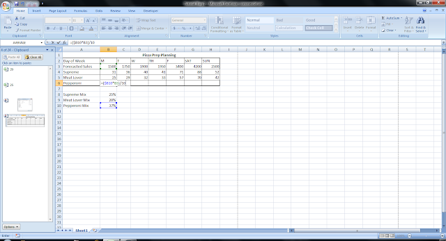
• In cell B6 place the formula =($B10*B3)/10. We will place a 10 in this formula because pepperoni pizzas are $2 cheaper than all others. Repeat decrease decimal and copy and paste. Below is an example of the formula:

Now that your spreadsheet is complete, you can change your forecasted sales or your mix percentage at any time. Since the formulas are already in place, it will change how many pizzas you need to make automatically. Your completed spreadsheet should look like this: